import libraries

from besos import eppy_funcs as ef, sampling
from besos.evaluator import EvaluatorEP
from besos.parameters import (
    FieldSelector,
    Parameter,
    RangeParameter,
    expand_plist,
    wwr,
)
from besos.problem import EPProblem
from matplotlib import pyplot as plt
from seaborn import heatmap, pairplot


plt.rcParams["figure.figsize"] = [8, 8]

Parametric Analysis

This notebook performs a parametric analysis of a building design using EnergyPlus and BESOS helper functions. We load a model from in.idf, define parameters to vary, set objectives,then run the model for all parameter combinations and plot the results.

The EnergyPlus evaulator object EvaluatorEP consists of an EPProblem (Parameters to modify and objectives to report) and a building model. A problem (problem = parameters + objectives) can be easily applied to any building model (evaluator = problem + building).

Each building is described by an .idf or epJSON file. In order to modify it programatically, we load it as a Python object using wrappers for EEPy.

If you are using the newer JSON format, then any JSON parsing library will work.

building = ef.get_building("in.idf")

Let’s check what materials are in the model. (Eppy’s documentation describes how to explore and modify the IDF object directly.)

[
    materials.Name for materials in building.idfobjects["MATERIAL"]
]  # get a list of the Name property of all IDF objects of class MATERIAL

['1/2IN Gypsum',
 '1IN Stucco',
 '8IN Concrete HW',
 'F08 Metal surface',
 'F16 Acoustic tile',
 'G01a 19mm gypsum board',
 'G05 25mm wood',
 'I01 25mm insulation board',
 'M11 100mm lightweight concrete',
 'MAT-CC05 4 HW CONCRETE',
 'Metal Decking',
 'Roof Insulation [18]',
 'Roof Membrane',
 'Wall Insulation [31]']

Selectors identify which part of the building model to modify and how to modify it (see the Selectors notebook for details). The Selector below specifies the Thickness field of an object named Mass NonRes Wall Insulation.

insulation = FieldSelector(
    class_name="Material", object_name="Wall Insulation [31]", field_name="Thickness"
)

Descriptors

Descriptors specify what values are valid for a parameter, see the Descriptors for details. If we want to vary a parameter \(0.01 \leq x \leq 0.99\), we can use a RangeParameter:

zero_to_one_exclusive = RangeParameter(min_val=0.01, max_val=0.99)

We can combine this with the Selector above to get a Parameter:

insulation_param = Parameter(
    selector=insulation,
    value_descriptor=zero_to_one_exclusive,
    name="Insulation Thickness",
)
print(insulation_param)

Parameter(selector=FieldSelector(field_name='Thickness', class_name='Material', object_name='Wall Insulation [31]'), value_descriptors=[RangeParameter(min=0.01, max=0.99)])

/home/user/.local/lib/python3.7/site-packages/besos/parameters.py:425: FutureWarning: Use value_descriptors instead of value_descriptor.
  FutureWarning("Use value_descriptors instead of value_descriptor.")

Short-cuts for defining parameters

The expand_plist funcion can define Parameters more concisely. It takes a nested dictionary as input. The keys in the first layer of this dictionary are the names of the idf objects. These are associated with a dictionary that has keys matching the Fields of that object to modify. Each field-key corresponds to a tuple containing the minimum and maximum values for that parameter. The class_name is not specified. Instead the model is searched for objects with the correct object_name. Note - doesn’t like duplicate object names!.

more_parameters = expand_plist(
    # class_name is NOT provided
    # {'object_name':
    # {'field_name':(min, max)}}
    {"Theoretical Glass [167]": {"Conductivity": (0.1, 5)}}
)

for p in more_parameters:
    print(p)

Parameter(selector=FieldSelector(field_name='Conductivity', object_name='Theoretical Glass [167]'), value_descriptors=[RangeParameter(name='Conductivity', min=0.1, max=5)])

Parameter scripts

BESOS also includes some pre-defined parameter scripts: + wwr(Range) for window to wall ratio

Here we define the WWR of all walls in the model to be between 10% and 90%.

window_to_wall = wwr(
    RangeParameter(0.1, 0.9)
)  # use a special shortcut to get the window-to-wall parameter

Custom parameter scripts

Parameters can also be created by defining a function that takes an idf and a value and mutates the idf. These functions can be specific to a certain idf file, and can perform any arbitrary transformation. Creating these can be more involved, and is not covered in this example.

Problems

Problem objects represent inputs and outputs. We have defined various inputs using parameters above, and we define objectives of heating and cooling use.

# Add all the parameters to a single parameters object.
parameters = [insulation_param] + more_parameters + [window_to_wall]

# Let us try to optimize the Cooling and the Heating of facility at the same time
objectives = ["DistrictCooling:Facility", "DistrictHeating:Facility"]
# These are hourly values, default is sum all the hourly values

# Construct the problem
problem = EPProblem(
    parameters, objectives
)  # Make a problem instance from the parameters and objectives

Sampling

Once you have defined your parameters, you may want to generate some random possible buildings. Sampling functions allow you to do this.

inputs = sampling.dist_sampler(sampling.full_factorial, problem, num_samples=5, level=2)
inputs

	Insulation Thickness	Conductivity	RangeParameter [0.1, 0.9]
0	0.01	0.10	0.1
1	0.50	0.10	0.1
2	0.01	2.55	0.1
3	0.50	2.55	0.1
4	0.01	0.10	0.5
5	0.50	0.10	0.5
6	0.01	2.55	0.5
7	0.50	2.55	0.5

inputs_lhs = sampling.dist_sampler(sampling.lhs, problem, num_samples=5)
inputs_lhs

	Insulation Thickness	Conductivity	RangeParameter [0.1, 0.9]
0	0.858166	4.962769	0.774880
1	0.592323	1.421850	0.460476
2	0.195969	2.483405	0.640751
3	0.702352	3.459438	0.285617
4	0.261383	0.780125	0.147248

Evaluation

Now we can evaluate the samples. We create an energy plus evaluator (EvaluatroEP) using the parameters, and idf describing the building, and the objectives we want to measure. For this example we will just use one of the premade objectives: Electricity use for the whole facility.

evaluator = EvaluatorEP(problem, building, out_dir="outputdir", err_dir="outputdir")
outputs = evaluator.df_apply(inputs, keep_input=True)

outputs.describe()

HBox(children=(FloatProgress(value=0.0, description='Executing', max=8.0, style=ProgressStyle(description_widt…

	Insulation Thickness	Conductivity	RangeParameter [0.1, 0.9]	DistrictCooling:Facility	DistrictHeating:Facility
count	8.000000	8.00000	8.000000	8.000000e+00	8.000000e+00
mean	0.255000	1.32500	0.300000	4.352905e+09	2.385049e+09
std	0.261916	1.30958	0.213809	2.137848e+08	1.460792e+09
min	0.010000	0.10000	0.100000	4.052084e+09	3.887300e+08
25%	0.010000	0.10000	0.100000	4.199775e+09	1.499059e+09
50%	0.255000	1.32500	0.300000	4.326841e+09	2.565410e+09
75%	0.500000	2.55000	0.500000	4.553878e+09	3.206888e+09
max	0.500000	2.55000	0.500000	4.615421e+09	4.356677e+09

Visualizing the results

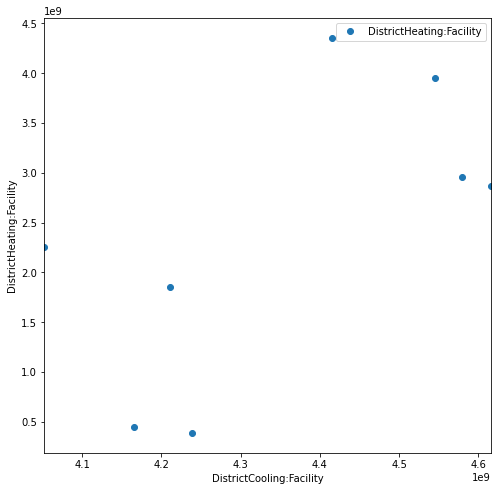
First we can see the variation in the objectives:

_ = outputs.plot(x=objectives[0], y=objectives[1], style="o")
plt.xlabel(objectives[0])
plt.ylabel(objectives[1])

Text(0, 0.5, 'DistrictHeating:Facility')

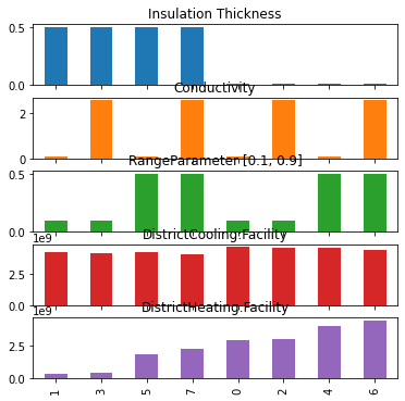
And compare the trends in the input values as the heating objective increases:

outputs = outputs.sort_values(by=objectives[1])
ax = outputs.plot.bar(subplots=True, legend=None, figsize=(6, 6))

/usr/local/lib/python3.7/dist-packages/pandas/plotting/_matplotlib/tools.py:307: MatplotlibDeprecationWarning:
The rowNum attribute was deprecated in Matplotlib 3.2 and will be removed two minor releases later. Use ax.get_subplotspec().rowspan.start instead.
  layout[ax.rowNum, ax.colNum] = ax.get_visible()
/usr/local/lib/python3.7/dist-packages/pandas/plotting/_matplotlib/tools.py:307: MatplotlibDeprecationWarning:
The colNum attribute was deprecated in Matplotlib 3.2 and will be removed two minor releases later. Use ax.get_subplotspec().colspan.start instead.
  layout[ax.rowNum, ax.colNum] = ax.get_visible()
/usr/local/lib/python3.7/dist-packages/pandas/plotting/_matplotlib/tools.py:313: MatplotlibDeprecationWarning:
The rowNum attribute was deprecated in Matplotlib 3.2 and will be removed two minor releases later. Use ax.get_subplotspec().rowspan.start instead.
  if not layout[ax.rowNum + 1, ax.colNum]:
/usr/local/lib/python3.7/dist-packages/pandas/plotting/_matplotlib/tools.py:313: MatplotlibDeprecationWarning:
The colNum attribute was deprecated in Matplotlib 3.2 and will be removed two minor releases later. Use ax.get_subplotspec().colspan.start instead.
  if not layout[ax.rowNum + 1, ax.colNum]:

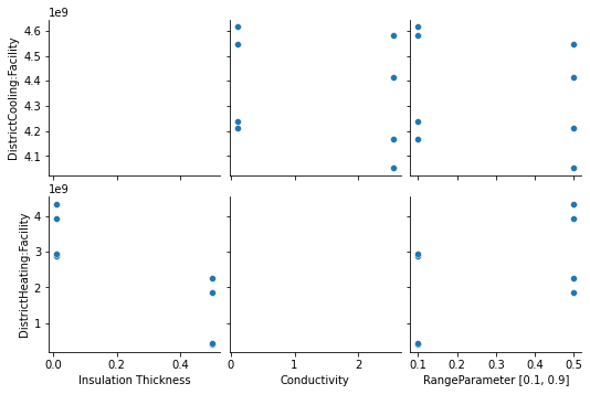
Visualising the parametric analysis

A better way to analyse the results is by looking at scatter plots of the inputs versus the outputs. This enables us to visually see strong relationships of inputs and outputs.

_ = pairplot(outputs, x_vars=inputs.columns, y_vars=objectives, kind="scatter")

Correlation heat map

Another way to analyse the impact of the inputs on the outputs is by analysing the correlation. A common metric is the Pearsson correlation coefficient:

$ r = :raw-latex:`\frac{N\sum{XY}-(\sum{X}\sum{Y})}{\sqrt{ [N\sum{x^2}-(\sum{x})^2 ][N\sum{y^2}-(\sum{y})^2 }]}` $

where N is the number of samples. \(X\) is the vector of observation of variable 1 (e.g. wall conductivity) and \(Y\) is the vetor of observations of variable 2 (e.g. electricity consumption). The closer \(r\) is to one the stronger the correlation, and similarly for negative one and negative correleation.

To visualize the correlation coefficients of all inputs and outputs, we can plot a heatmap:

_ = heatmap(outputs.corr())

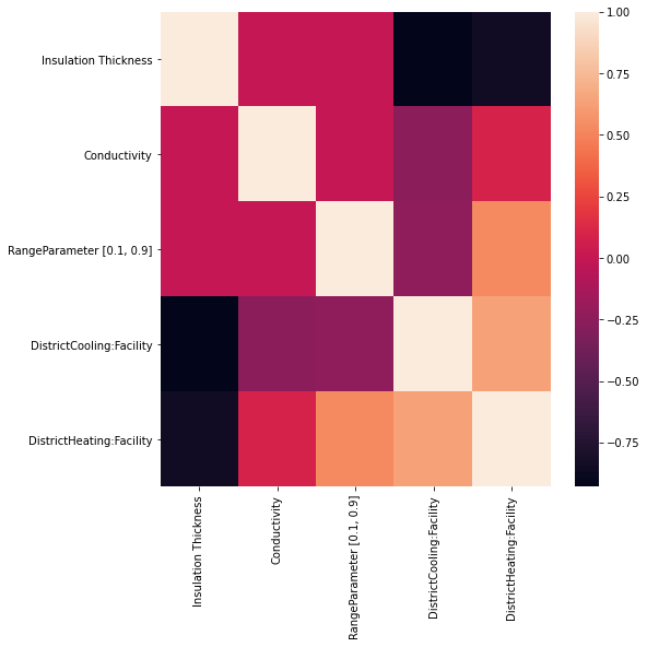
The heatmap shows well that the impact of ‘Equipment’ and ‘Lighting’ is the most important given this example of an office building. The U-Value and the attic insultation thickness have suprisingly little effect.