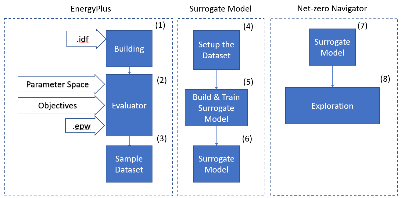
Example Work Flow
Warning
To run this example you will need to install TensorFlow which is >300mb library. To install run pip install tensorflow
Note
Lots of other great surrogate modelling examples can be found here that make use of scikit learn instead of TensorFlow.
In this notebook we will go over a ensemble model made possible by the besos software. We will create a surrogate model of a parameterized EnergyPlus building model. The model is changed based on a given window to wall ratio and solar gain coefficient. These variables will change the daily electricity use of the buildings. We will create a dataset of different buildings that will contain the variations of parameters and a time series of daily electricity use. Using this dataset we will train a neural network to quickly find those daily electricity values without the need to rerun the EnergyPlus model. Finally we will use this surrogate model to explore the impact of the variables using a parallel coordinates plot. To complete this we will walk through nine steps as seen in the figure below.
First we will import all the different libraries we need.
#!pip install besos --user
%matplotlib inline

import pandas as pd
import numpy as np
import tensorflow as tf
import tensorflow.keras as keras
from tensorflow.keras import layers
from besos import eppy_funcs as ef
import besos.sampling as sampling
from besos.problem import EPProblem
from besos.evaluator import EvaluatorEP
from besos.parameters import wwr, RangeParameter,FieldSelector, Parameter
import tensorflow_docs as tfdocs
import tensorflow_docs.plots
import tensorflow_docs.modeling
import time
from dask.distributed import Client
# Use seaborn for pairplot
#!pip install --upgrade tensorflow --user

# Use some functions from tensorflow_docs
#!pip install git+https://github.com/tensorflow/docs --user
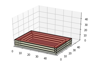
(1) Set up the building from idf
The building is defined by the Information Data File (IDF) or using the new EnergyPlus format (epJSON).
# Open the IDF file
building = ef.get_building("./examples/EnsembleWorkflows/Medium_Office.idf")
building.view_model()
#You can convert an idf to epJSON using the following code.
# !energyplus -c "/examples/EnsembleWorkflows/Medium_Office.idf"
(2) Evaluator
Set up the inputs and outputs of your exploration
Defines how we will evaluate the building; - what external weather conditions is the building experiencing, - what properties of the building will we be changing, and - what are some of the performance metrics of the building that we want to explore.
The weather conditions are specified in the EnergyPlus Weather File (EWP) file. The properties we will change in the building will be defined in the parameter space. In the objectives we will specify the what output performance metrics we wish to extract such that we can explore them later.
# building.idfobjects
# for materials in building.idfobjects["MATERIAL:NOMASS"]:
#     print("{} {}".format(materials.Name,materials.Thermal_Resistance))

# for materials in building.idfobjects["BUILDINGSURFACE:DETAILED"]:
#     if materials.Sun_Exposure!="NoSun": print(materials.Construction_Name )

# for materials in building.idfobjects['CONSTRUCTION']:
#     if materials.Name=="BTAP-Ext-Wall-Mass:U-0.315": print(materials)

Figure 2: Setting up the evaluator
# Here we change all the external insulation of the building
insu1 = FieldSelector(class_name='MATERIAL:NOMASS', object_name='Typical Insulation 2', field_name='Thermal Resistance')


# Setup the parameters, Solar Heat Gain Coefficient
parameters = [Parameter(FieldSelector('Window',"*",'Solar Heat Gain Coefficient'),
                value_descriptor=RangeParameter(0.01,0.99),
                name='Solar Gain Coefficient'),
             Parameter(insu1,
                value_descriptor=RangeParameter(1,15),
                name='Insulation Resistance'),]


# Add window-to-wall ratio as a parameter between 0.1 and 0.9 using a custom function
parameters.append(wwr(RangeParameter(0.1, 0.9)))


# Construct the objective
objective = ['Electricity:Facility']


# Build the problem
problem = EPProblem(parameters, objective)
# setup the evaluator
evaluator = EvaluatorEP(problem, building, epw_file = "/examples/EnsembleWorkflows/victoria.epw", multi=True,
                        progress_bar=True, distributed=True, out_dir="outputdirectory")
(3) Generate the Dataset
Sample the problem space
Setup the parallel processing
Generate the Samples
Store and recover the expensive runs
# Use latin hypercube sampling to take 30 samples
inputs = sampling.dist_sampler(sampling.lhs, problem,100)


# sample of the inputs
print(inputs.head())
   Solar Gain Coefficient  Insulation Resistance  Window to Wall Ratio
0                0.980214               9.160124              0.650856
1                0.661204              13.430512              0.597784
2                0.716411               4.617035              0.337802
3                0.518645               7.229073              0.677144
4                0.206976              10.194319              0.808266
# Setup the parallel processing in the notebook.
client = Client(threads_per_worker=1)
client
Client
|
Cluster
|
Run the samples
t1=time.time()
# Run Energyplus
outputs = evaluator.df_apply(inputs)
t2=time.time()
time_of_sim=t2-t1
/usr/local/lib/python3.7/dist-packages/distributed/worker.py:3339: UserWarning: Large object of size 6.95 MB detected in task graph:
  ("('from_pandas-10fc1b0e937cec3185233c4f9719f146', ... 33c4f9719f146')
Consider scattering large objects ahead of time
with client.scatter to reduce scheduler burden and
keep data on workers

    future = client.submit(func, big_data)    # bad

    big_future = client.scatter(big_data)     # good
    future = client.submit(func, big_future)  # good
  % (format_bytes(len(b)), s)
Calculate the time
def niceformat(seconds):
    seconds = seconds % (24 * 3600)
    hour = seconds // 3600
    seconds %= 3600
    minutes = seconds // 60
    seconds %= 60
    return hour, minutes, seconds

hours,mins,secs=niceformat(time_of_sim)

print("The total running time: {:2.0f} hours {:2.0f} min {:2.0f} seconds".format(hours,mins,secs))
# Build a results DataFrame
results = inputs.join(outputs)
results.head()
Take a look at the results
total_heating_use = results['Electricity:Facility']

def norm_res(results):
    results_normed = (results - np.mean(results))/np.std(results)
    return results_normed

plt.scatter(norm_res(results['Solar Gain Coefficient']),total_heating_use,label="solar gain")
plt.scatter(norm_res(results['Window to Wall Ratio']),total_heating_use,label="w2w ratio")
plt.scatter(norm_res(results['Insulation Resistance']),total_heating_use,label="Insulation Resistance")

plt.legend()
Store the expensive calculations
Since this can quite a big run. Lets store the results such that we don’t have to rerun this problem.
inputs.to_pickle("inputs.pkl")
outputs.to_pickle("outputs.pkl")
inputs_ = pd.read_pickle("inputs.pkl")
outputs_ = pd.read_pickle("outputs.pkl")
(4) Setup the dataset for the Surrogate Model
The outputs are packed in a single columns which will not work for tensorflow.
print(outputs_.head())
print(inputs_.head())
   Electricity:Facility
0          1.999243e+12
1          1.966446e+12
2          1.634494e+12
3          1.604978e+12
4          1.838792e+12
   Solar Gain Coefficient  Insulation Resistance  Window to Wall Ratio
0                0.908584               4.854668              0.822617
1                0.469324              11.766597              0.798576
2                0.390397               7.866908              0.188102
3                0.367993               9.632202              0.120128
4                0.405527               9.803255              0.585378
We will repack them using the following code, to get 365 different columns which will represent the output labels. Build the full dataset with inputs and outputs to easily split up the train and test data sets. The training data sets are used to train the model, while the test data set will show how general the model is.
dataset=inputs_.join(outputs_)
dataset.head()
| Solar Gain Coefficient | Insulation Resistance | Window to Wall Ratio | Electricity:Facility | |
|---|---|---|---|---|
| 0 | 0.908584 | 4.854668 | 0.822617 | 1.999243e+12 |
| 1 | 0.469324 | 11.766597 | 0.798576 | 1.966446e+12 |
| 2 | 0.390397 | 7.866908 | 0.188102 | 1.634494e+12 |
| 3 | 0.367993 | 9.632202 | 0.120128 | 1.604978e+12 |
| 4 | 0.405527 | 9.803255 | 0.585378 | 1.838792e+12 |
Split dataset into test and training
train_dataset = dataset.sample(frac=0.8, random_state=0)
test_dataset = dataset.drop(train_dataset.index)

training_labels = train_dataset[outputs_.columns]
testing_labels = test_dataset[outputs_.columns]
training_labels
| Electricity:Facility | |
|---|---|
| 26 | 1.954075e+12 |
| 86 | 1.710905e+12 |
| 2 | 1.634494e+12 |
| 55 | 1.724594e+12 |
| 75 | 1.722192e+12 |
| ... | ... |
| 69 | 1.724147e+12 |
| 20 | 1.949339e+12 |
| 94 | 1.921412e+12 |
| 72 | 1.758905e+12 |
| 77 | 1.885642e+12 |
80 rows × 1 columns
Normalize the Data (Inputs of the model)
We will normalize the inputs and the outputs
train_stats = train_dataset[inputs_.columns]
train_stats = train_stats.describe()
train_stats = train_stats.transpose()
train_stats
| count | mean | std | min | 25% | 50% | 75% | max | |
|---|---|---|---|---|---|---|---|---|
| Solar Gain Coefficient | 80.0 | 0.519140 | 0.269162 | 0.015683 | 0.302935 | 0.527331 | 0.735092 | 0.988500 |
| Insulation Resistance | 80.0 | 7.822454 | 4.022222 | 1.124960 | 4.420202 | 7.855031 | 10.947344 | 14.994939 |
| Window to Wall Ratio | 80.0 | 0.508981 | 0.222432 | 0.111234 | 0.332921 | 0.510361 | 0.697192 | 0.885781 |
# use the stats we calculated to do the normalization on the input.
def norm_input(x):
    return (x - train_stats['mean']) / train_stats['std']

def unnorm_input(x):
    return (x* train_stats['std'])+ train_stats['mean']

normed_train_data = norm_input(train_dataset[inputs_.columns])
normed_test_data = norm_input(test_dataset[inputs_.columns])


print(test_dataset[inputs_.columns].head())
print(normed_test_data.head())
print(unnorm_input(normed_test_data.head()))
    Solar Gain Coefficient  Insulation Resistance  Window to Wall Ratio
9                 0.807155               6.023020              0.465111
12                0.663061              12.758043              0.541317
21                0.865366              11.065040              0.736124
25                0.164315               1.926658              0.242456
36                0.251987               5.551554              0.330283
    Solar Gain Coefficient  Insulation Resistance  Window to Wall Ratio
9                 1.070047              -0.447373             -0.197232
12                0.534702               1.227080              0.145375
21                1.286313               0.806168              1.021179
25               -1.318257              -1.465806             -1.198237
36               -0.992535              -0.564589             -0.803388
    Solar Gain Coefficient  Insulation Resistance  Window to Wall Ratio
9                 0.807155               6.023020              0.465111
12                0.663061              12.758043              0.541317
21                0.865366              11.065040              0.736124
25                0.164315               1.926658              0.242456
36                0.251987               5.551554              0.330283
Normalize the labels (Outputs of the model)
labels are the actual outputs that we are interested in.
train_mean = np.mean(training_labels)
train_std  = np.std(testing_labels)
train_mean, train_std
(Electricity:Facility    1.816284e+12
 dtype: float64,
 Electricity:Facility    1.433704e+11
 dtype: float64)
def norm_output(x):
    return (x - train_mean) /train_std

def unnorm_output(x):
    return (x*train_std)+ train_mean

train_labels = norm_output(training_labels)
test_labels  = norm_output(testing_labels)
train_labels.head()
| Electricity:Facility | |
|---|---|
| 26 | 0.961087 |
| 86 | -0.735008 |
| 2 | -1.267970 |
| 55 | -0.639533 |
| 75 | -0.656285 |
(5) Build & Train Surrogate model architecture
def build_model():
    model = keras.Sequential([
       layers.Dense(5, input_shape=[len(train_dataset[inputs_.columns].keys())]),
       layers.Dense(5),
       layers.Dense(1)
    ])

    optimizer = tf.keras.optimizers.RMSprop(0.0001)

    model.compile(loss='mse',
                optimizer=optimizer,
                metrics=['mae', 'mse'])
    return model
model = build_model()
model.summary()
Model: "sequential"
_________________________________________________________________
Layer (type)                 Output Shape              Param #
=================================================================
dense (Dense)                (None, 5)                 20
_________________________________________________________________
dense_1 (Dense)              (None, 5)                 30
_________________________________________________________________
dense_2 (Dense)              (None, 1)                 6
=================================================================
Total params: 56
Trainable params: 56
Non-trainable params: 0
_________________________________________________________________
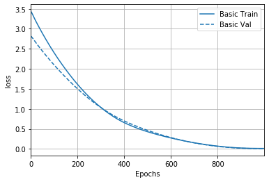
EPOCHS = 1000

history = model.fit(
  normed_train_data, train_labels,
  epochs=EPOCHS, validation_split = 0.2, verbose=0,
  callbacks=[tfdocs.modeling.EpochDots()])
Epoch: 0, loss:3.4908,  mae:1.5995,  mse:3.4908,  val_loss:2.8472,  val_mae:1.4809,  val_mse:2.8472,
....................................................................................................
Epoch: 100, loss:2.4005,  mae:1.3447,  mse:2.4005,  val_loss:2.0969,  val_mae:1.2491,  val_mse:2.0969,
....................................................................................................
Epoch: 200, loss:1.6133,  mae:1.1169,  mse:1.6133,  val_loss:1.5025,  val_mae:1.0296,  val_mse:1.5025,
....................................................................................................
Epoch: 300, loss:1.0368,  mae:0.9047,  mse:1.0368,  val_loss:1.0345,  val_mae:0.8159,  val_mse:1.0345,
....................................................................................................
Epoch: 400, loss:0.6570,  mae:0.7113,  mse:0.6570,  val_loss:0.7000,  val_mae:0.6246,  val_mse:0.7000,
....................................................................................................
Epoch: 500, loss:0.4305,  mae:0.5583,  mse:0.4305,  val_loss:0.4642,  val_mae:0.4929,  val_mse:0.4642,
....................................................................................................
Epoch: 600, loss:0.2742,  mae:0.4388,  mse:0.2742,  val_loss:0.2843,  val_mae:0.3906,  val_mse:0.2843,
....................................................................................................
Epoch: 700, loss:0.1550,  mae:0.3292,  mse:0.1550,  val_loss:0.1515,  val_mae:0.2824,  val_mse:0.1515,
....................................................................................................
Epoch: 800, loss:0.0707,  mae:0.2218,  mse:0.0707,  val_loss:0.0645,  val_mae:0.1818,  val_mse:0.0645,
....................................................................................................
Epoch: 900, loss:0.0242,  mae:0.1210,  mse:0.0242,  val_loss:0.0191,  val_mae:0.0999,  val_mse:0.0191,
....................................................................................................
plotter = tfdocs.plots.HistoryPlotter(smoothing_std=2)
plotter.plot({'Basic': history}, metric = "loss")
plt.ylabel('loss')
Text(0, 0.5, 'loss')
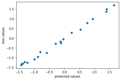
(6) Surrogate Model & Validate against the Test dataset
# See -> https://en.wikipedia.org/wiki/Coefficient_of_determination
# R squared score:
r_sqared_scores = []
sum_res_s = []
sum_tot_s = []
y_i = test_labels.loc[test_labels.index].values
y_m = np.mean(y_i)/y_i.size
for i in range(len(normed_test_data)):
    x_i = normed_test_data.loc[normed_test_data.index[i]].tolist()
    f_i = model.predict([x_i])[0]
    y_i = test_labels.loc[test_labels.index[i]].values
    ss_res=(f_i-y_i)**2
    ss_tot=(y_i-y_m)**2
    sum_res_s.append(f_i)
    sum_tot_s.append(y_i)
    r_sqared_scores.append(1-ss_res/ss_tot)

plt.scatter(sum_res_s,sum_tot_s)
plt.xlabel("predicted values")
plt.ylabel("test values")
print("average R sqaured score: {}".format(np.mean(r_sqared_scores)))
average R sqaured score: 0.9704462861305323
(7) Sample Surrogate Model
from besos.evaluator import EvaluatorGeneric
def evaluation_func(ind):
    vals = norm_input(list(ind))
    output = unnorm_output(model.predict([list(vals)])[0][0])
    return ((output.values[0],),())

GP_SM = EvaluatorGeneric(evaluation_func, problem)
srinputs = sampling.dist_sampler(sampling.lhs, problem, 100)
sroutputs = GP_SM.df_apply(srinputs)
srresults = srinputs.join(sroutputs)
srresults.head()
HBox(children=(FloatProgress(value=0.0, description='Executing', style=ProgressStyle(description_width='initia…
| Solar Gain Coefficient | Insulation Resistance | Window to Wall Ratio | Electricity:Facility | |
|---|---|---|---|---|
| 0 | 0.877723 | 10.328806 | 0.151321 | 1.602558e+12 |
| 1 | 0.430164 | 6.025796 | 0.384092 | 1.757320e+12 |
| 2 | 0.561125 | 9.407312 | 0.777024 | 1.958208e+12 |
| 3 | 0.086388 | 14.182918 | 0.141822 | 1.587385e+12 |
| 4 | 0.303898 | 7.201950 | 0.896001 | 2.037647e+12 |
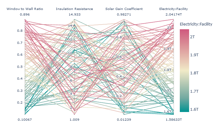
(8) Exploration
import plotly
plotly.offline.init_notebook_mode(connected=True)
import plotly.express as px
fig = px.parallel_coordinates(srresults,color="Electricity:Facility", dimensions=["Window to Wall Ratio",
                "Insulation Resistance","Solar Gain Coefficient" ,"Electricity:Facility"],
                             color_continuous_scale=px.colors.diverging.Tealrose)
fig.show()