Adaptive Sampling
This notebook implements adaptive sampling, which explores under-sampled parts of the design space while exploiting the knowledge gained from previous simulation runs. The aim is to reduce the number of samples required to train an accurate surrogate model. We use Lola-Voronoi based sampling, which is compatible with any surrogate model type. Here it is applied with a Gaussian Process model.
import warnings

import numpy as np
import seaborn as sns
from besos import eppy_funcs as ef, sampling
from besos.evaluator import EvaluatorEP
from besos.problem import EPProblem
from dask.distributed import Client
from matplotlib import pyplot as plt
from scipy.interpolate import griddata
from sklearn.gaussian_process import GaussianProcessRegressor
from sklearn.gaussian_process.kernels import RBF, Matern, RationalQuadratic
from sklearn.manifold import MDS
from sklearn.model_selection import GridSearchCV, train_test_split
from sklearn.preprocessing import StandardScaler

from parameter_sets import parameter_set
from sampling import adaptive_sampler_lv
client = Client(threads_per_worker=1)
client
Client
|
Cluster
|
Define sampler settings
n_samples_init = (
    20  # initial set of samples collected using the standard low-discrepancy sampling
)

no_iter = 10  # number of iterations of the adaptive sampler to run
n = 4  # number of samples added per iteration
Generate data set
This generates an example model and the initial sampling data, see this example.
parameters = parameter_set(7)
problem = EPProblem(parameters, ["Electricity:Facility"])
building = ef.get_building()
inputs = sampling.dist_sampler(sampling.lhs, problem, n_samples_init)
evaluator = EvaluatorEP(problem, building)
outputs = evaluator.df_apply(inputs, processes=4)
results = inputs.join(outputs)
results.head()
| Conductivity | Thickness | U-Factor | Solar Heat Gain Coefficient | ElectricEquipment | Lights | Window to Wall Ratio | Electricity:Facility | |
|---|---|---|---|---|---|---|---|---|
| 0 | 0.068922 | 0.278260 | 0.589089 | 0.808344 | 11.278208 | 12.836307 | 0.114060 | 1.994176e+09 |
| 1 | 0.165364 | 0.199395 | 2.800824 | 0.907124 | 10.950859 | 10.328810 | 0.502100 | 1.845950e+09 |
| 2 | 0.159571 | 0.249230 | 0.290241 | 0.980416 | 14.532254 | 11.521821 | 0.884315 | 2.152789e+09 |
| 3 | 0.083254 | 0.112736 | 1.924484 | 0.297179 | 14.368944 | 12.232532 | 0.804670 | 2.119206e+09 |
| 4 | 0.028942 | 0.203402 | 4.931487 | 0.079449 | 11.817406 | 14.989872 | 0.679059 | 2.103819e+09 |
Initial training of Surrogate Model
Here we use a Gaussian Process surrogate model, see here for details.
train_in, test_in, train_out, test_out = train_test_split(
    inputs, outputs, test_size=0.2
)
hyperparameters = {
    "kernel": [
        None,
        1.0 * RBF(length_scale=1.0, length_scale_bounds=(1e-1, 10.0)),
        1.0 * RationalQuadratic(length_scale=1.0, alpha=0.5),
        # ConstantKernel(0.1, (0.01, 10.0))*(DotProduct(sigma_0=1.0, sigma_0_bounds=(0.1, 10.0))**2),
        1.0 * Matern(length_scale=1.0, length_scale_bounds=(1e-1, 10.0)),
    ]
}

folds = 3

gp = GaussianProcessRegressor(normalize_y=True)

clf = GridSearchCV(gp, hyperparameters, iid=True, cv=folds)
with warnings.catch_warnings():
    warnings.simplefilter("ignore", category=FutureWarning)
    clf.fit(inputs, outputs)

print(f"The best performing model $R^2$ score on the validation set: {clf.best_score_}")
print(f"The model $R^2$ parameters: {clf.best_params_}")
print(
    f"The best performing model $R^2$ score on a separate test set: {clf.best_estimator_.score(test_in, test_out)}"
)
reg = clf.best_estimator_
The best performing model $R^2$ score on the validation set: 0.8932778938504393
The model $R^2$ parameters: {'kernel': 1**2 * Matern(length_scale=1, nu=1.5)}
The best performing model $R^2$ score on a separate test set: 1.0
LOLA - Voronoi sampling
Here we run our implementation of LOLA-Voronoi sampling. New designs to be simulated are picked around previously simulated designs with a high hybrid score \(H\).
\(H = V + E\)
\(H\) is used to incentives exploration \(V\) and exploitation \(E\). \(V\) is the Voronoi cell size to approximate the sample density and \(E\) the local-linear estimate to approximate the gradient in the neighbourhood of a sample.
numiter = 10
AS = adaptive_sampler_lv(
    train_in.values,
    train_out.values,
    n,
    problem,
    evaluator,
    reg,
    test_in,
    test_out,
    verbose=False,
)
AS.run(numiter)
HBox(children=(FloatProgress(value=0.0, description='Executing', max=4.0, style=ProgressStyle(description_widt…
0
HBox(children=(FloatProgress(value=0.0, description='Executing', max=4.0, style=ProgressStyle(description_widt…
1
HBox(children=(FloatProgress(value=0.0, description='Executing', max=4.0, style=ProgressStyle(description_widt…
2
/home/user/.local/lib/python3.7/site-packages/sklearn/gaussian_process/_gpr.py:504: ConvergenceWarning: lbfgs failed to converge (status=2):
ABNORMAL_TERMINATION_IN_LNSRCH.

Increase the number of iterations (max_iter) or scale the data as shown in:
    https://scikit-learn.org/stable/modules/preprocessing.html
  _check_optimize_result("lbfgs", opt_res)
HBox(children=(FloatProgress(value=0.0, description='Executing', max=4.0, style=ProgressStyle(description_widt…
3
HBox(children=(FloatProgress(value=0.0, description='Executing', max=4.0, style=ProgressStyle(description_widt…
4
HBox(children=(FloatProgress(value=0.0, description='Executing', max=4.0, style=ProgressStyle(description_widt…
5
HBox(children=(FloatProgress(value=0.0, description='Executing', max=4.0, style=ProgressStyle(description_widt…
6
HBox(children=(FloatProgress(value=0.0, description='Executing', max=4.0, style=ProgressStyle(description_widt…
7
HBox(children=(FloatProgress(value=0.0, description='Executing', max=4.0, style=ProgressStyle(description_widt…
8
HBox(children=(FloatProgress(value=0.0, description='Executing', max=4.0, style=ProgressStyle(description_widt…
9
HBox(children=(FloatProgress(value=0.0, description='Executing', max=4.0, style=ProgressStyle(description_widt…
/home/user/.local/lib/python3.7/site-packages/sklearn/gaussian_process/_gpr.py:504: ConvergenceWarning: lbfgs failed to converge (status=2):
ABNORMAL_TERMINATION_IN_LNSRCH.

Increase the number of iterations (max_iter) or scale the data as shown in:
    https://scikit-learn.org/stable/modules/preprocessing.html
  _check_optimize_result("lbfgs", opt_res)
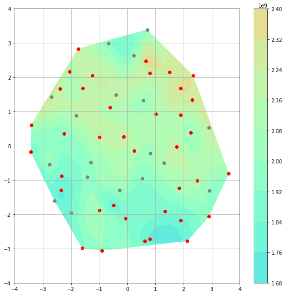
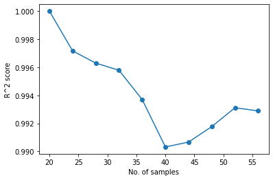
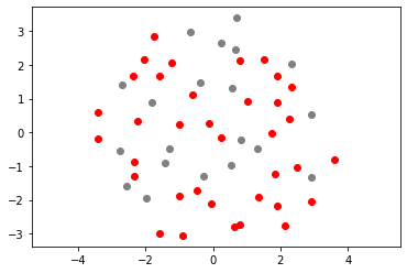
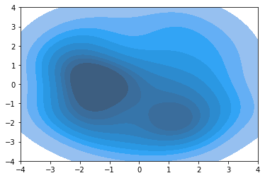
Visualization
We visualize the working of the adaptive sampler by reducing the input dimensionality to 2 using multi-dimensional scaling.
plt.plot(range(n_samples_init, n_samples_init + no_iter * n, n), AS.score[:-1], "-o")
plt.ylabel("R^2 score")
plt.xlabel("No. of samples")
Text(0.5, 0, 'No. of samples')
# Manifold model
scaler_mds = StandardScaler()
p_norm = scaler_mds.fit_transform(AS.P)
model = MDS(n_components=2, random_state=1)
out3 = model.fit_transform(p_norm)

plt.scatter(out3[:n_samples_init, 0], out3[:n_samples_init, 1], color="grey")
plt.scatter(out3[n_samples_init:, 0], out3[n_samples_init:, 1], color="r")
plt.axis("equal")
(-4.207227499374288, 4.505355347028606, -3.7690514453462707, 4.057620752975868)
ax = sns.kdeplot(out3[n_samples_init:, 0], out3[n_samples_init:, 1], shade=True)
plt.ylim([-4, 4])
plt.xlim([-4, 4])
/usr/local/lib/python3.7/dist-packages/seaborn/_decorators.py:43: FutureWarning: Pass the following variable as a keyword arg: y. From version 0.12, the only valid positional argument will be data, and passing other arguments without an explicit keyword will result in an error or misinterpretation.
  FutureWarning
(-4.0, 4.0)
x = out3[:, 0]
y = out3[:, 1]
z = reg.predict(AS.P)

# Convert from pandas dataframes to numpy arrays
X, Y, Z, = np.array([]), np.array([]), np.array([])
for i in range(len(x)):
    X = np.append(X, x[i])
    Y = np.append(Y, y[i])
    Z = np.append(Z, z[i])

# create x-y points to be used in heatmap
xi = np.linspace(X.min(), X.max(), 1000)
yi = np.linspace(Y.min(), Y.max(), 1000)

# Z is a matrix of x-y values
zi = griddata((X, Y), Z, (xi[None, :], yi[:, None]), method="cubic")

# I control the range of my colorbar by removing data
# outside of my range of interest
zmin = 1.0 * 10 ** 9
zmax = 3 * 10 ** 9
zi[(zi < zmin) | (zi > zmax)] = None

# Create the contour plot
plt.figure(figsize=(10, 10))
CS = plt.contourf(xi, yi, zi, 10, cmap=plt.cm.rainbow, vmax=zmax, vmin=zmin, alpha=0.8)
plt.colorbar()
plt.scatter(out3[:18, 0], out3[:18, 1], color="grey")
plt.scatter(out3[18:, 0], out3[18:, 1], color="r")
# ax = sns.kdeplot(out3[18:,0], out3[18:,1], shade=True)


plt.ylim([-4, 4])
plt.xlim([-4, 4])
plt.grid()
/usr/local/lib/python3.7/dist-packages/ipykernel_launcher.py:23: RuntimeWarning: invalid value encountered in less
/usr/local/lib/python3.7/dist-packages/ipykernel_launcher.py:23: RuntimeWarning: invalid value encountered in greater