Interactive Surrogate Modelling

In this notebook we: + define a problem consisting of parameters to vary with ranges and an objective function + sample the problem space + define an Evaluator by linking the problem to an EnergyPlus model + run the Evaluator for the samples + train a surrogate model over the samples + explore the design space using an interactive plot that queries the surrogate model

import numpy as np
import pandas as pd
import seaborn as sns
from besos import eppy_funcs as ef, sampling
from besos.evaluator import EvaluatorEP
from besos.parameters import FieldSelector, Parameter, RangeParameter
from besos.problem import EPProblem
from ipywidgets import FloatSlider, interact
from matplotlib import pyplot as plt
from sklearn import linear_model, pipeline
from sklearn.preprocessing import StandardScaler

Parameters and Objectives

We start by defining Parameters that govern how we would like to modify the building. Here they are the solar heat gain coefficient and the lighting power density.

parameters = [
    Parameter(
        FieldSelector(
            object_name="NonRes Fixed Assembly Window",
            field_name="Solar Heat Gain Coefficient",
        ),
        value_descriptor=RangeParameter(0.01, 0.99),
    ),
    Parameter(
        FieldSelector("Lights", "*", "Watts per Zone Floor Area"),
        value_descriptor=RangeParameter(8, 12),
        name="Lights Watts/Area",
    ),
]

/home/user/.local/lib/python3.7/site-packages/besos/parameters.py:425: FutureWarning: Use value_descriptors instead of value_descriptor.
  FutureWarning("Use value_descriptors instead of value_descriptor.")

Now, we specify that we would like to optimize for electricity use of the entire facility. We then bundle all of this information together.

objectives = ["Electricity:Facility"]

problem = EPProblem(parameters, objectives)

Sampling

We need to generate samples on which to train a surrogate model. The sampler uses Latin Hypercube Sampling to distribute the samples in the design space defined by the Parameters. We can check how well distributed they are using describe().

inputs = sampling.dist_sampler(sampling.lhs, problem, 5)
inputs.describe()  # properties of the sample set

	RangeParameter [0.01, 0.99]	Lights Watts/Area
count	5.000000	5.000000
mean	0.526836	10.015865
std	0.346252	1.455874
min	0.168450	8.067549
25%	0.225623	9.405653
50%	0.486488	9.821539
75%	0.793737	10.900807
max	0.959882	11.883777

Building model

Next we load an EnergyPlus model. The example is a small office, or we could pass in the IDF filename.

building = ef.get_building()

Evaluator

We now define and run the Evaluator, which will run the EnergyPlus instances with the different inputs generated in the previous cell.

evaluator = EvaluatorEP(problem, building)
train = evaluator.df_apply(inputs, keep_input=True)
train.head()  # first 5 lines

HBox(children=(FloatProgress(value=0.0, description='Executing', max=5.0, style=ProgressStyle(description_widt…

	RangeParameter [0.01, 0.99]	Lights Watts/Area	Electricity:Facility
0	0.793737	9.405653	1.928249e+09
1	0.168450	9.821539	1.734335e+09
2	0.486488	11.883777	1.954911e+09
3	0.959882	8.067549	1.910631e+09
4	0.225623	10.900807	1.820579e+09

We can save results at this point:

train.to_pickle("samples.p")

And load them again later:

train = pd.read_pickle("samples.p")

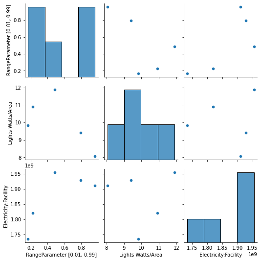
Exploring the training data

Let’s look at the correlation amongst the inputs and the output using a built-in Seaborn plot:

g = sns.pairplot(train)

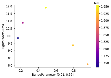
Here’s a plot of the design space defined by the samples.

x, y, obj = problem.names()
train.plot.hexbin(x=x, y=y, C=obj, cmap="plasma", sharex=False, gridsize=50)

/usr/local/lib/python3.7/dist-packages/pandas/plotting/_matplotlib/tools.py:307: MatplotlibDeprecationWarning:
The rowNum attribute was deprecated in Matplotlib 3.2 and will be removed two minor releases later. Use ax.get_subplotspec().rowspan.start instead.
  layout[ax.rowNum, ax.colNum] = ax.get_visible()
/usr/local/lib/python3.7/dist-packages/pandas/plotting/_matplotlib/tools.py:307: MatplotlibDeprecationWarning:
The colNum attribute was deprecated in Matplotlib 3.2 and will be removed two minor releases later. Use ax.get_subplotspec().colspan.start instead.
  layout[ax.rowNum, ax.colNum] = ax.get_visible()
/usr/local/lib/python3.7/dist-packages/pandas/plotting/_matplotlib/tools.py:313: MatplotlibDeprecationWarning:
The rowNum attribute was deprecated in Matplotlib 3.2 and will be removed two minor releases later. Use ax.get_subplotspec().rowspan.start instead.
  if not layout[ax.rowNum + 1, ax.colNum]:
/usr/local/lib/python3.7/dist-packages/pandas/plotting/_matplotlib/tools.py:313: MatplotlibDeprecationWarning:
The colNum attribute was deprecated in Matplotlib 3.2 and will be removed two minor releases later. Use ax.get_subplotspec().colspan.start instead.
  if not layout[ax.rowNum + 1, ax.colNum]:

<matplotlib.axes._subplots.AxesSubplot at 0x7f09fc0e1d90>

Fitting a surrogate model

Now we can train the model using a ScikitLearn pipeline:

model = pipeline.make_pipeline(StandardScaler(), linear_model.Ridge())
model.fit(train[[x, y]].values, train[obj].values)

Pipeline(steps=[('standardscaler', StandardScaler()), ('ridge', Ridge())])

Running the surrogate model

We can query the model at a specific point in the design space:

model.predict([[0.5, 10]])

array([1.86298733e+09])

Or for a dataframe made from a dictionary of points:

points = pd.DataFrame(data={"SHGC": [0, 1], "LPD": [8, 12]})
model.predict(points)

array([1.68282942e+09, 2.04314525e+09])

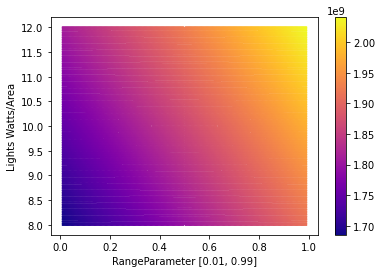
Next we define a function for querying the surrogate model across the domain at a given density, and plot the result.

def run_model(model, density):
    p1 = problem.inputs[0].value_descriptor
    a = np.linspace(p1.min, p1.max, density)
    p2 = problem.inputs[1].value_descriptor
    b = np.linspace(p2.min, p2.max, density)
    plot_data = pd.DataFrame(
        np.transpose([np.tile(a, len(b)), np.repeat(b, len(a))]),
        columns=problem.names("inputs"),
    )
    return pd.concat([plot_data, pd.Series(model.predict(plot_data))], axis=1)


density = 200
df = run_model(model, density)
df.plot.hexbin(x=x, y=y, C=0, cmap="plasma", gridsize=density, sharex=False)

/usr/local/lib/python3.7/dist-packages/ipykernel_launcher.py:2: DeprecationWarning: Call to deprecated function (or staticmethod) inputs. (Problem.inputs is ambiguous, use .value_descriptors or .parameters instead.) -- Deprecated since version 2.0.

/usr/local/lib/python3.7/dist-packages/ipykernel_launcher.py:2: DeprecationWarning: Call to deprecated function (or staticmethod) value_descriptor. (Does not support multiple Descriptors per Parameter.Use the value_descriptors of this Parameter instead.)

/usr/local/lib/python3.7/dist-packages/ipykernel_launcher.py:4: DeprecationWarning: Call to deprecated function (or staticmethod) inputs. (Problem.inputs is ambiguous, use .value_descriptors or .parameters instead.) -- Deprecated since version 2.0.
  after removing the cwd from sys.path.
/usr/local/lib/python3.7/dist-packages/ipykernel_launcher.py:4: DeprecationWarning: Call to deprecated function (or staticmethod) value_descriptor. (Does not support multiple Descriptors per Parameter.Use the value_descriptors of this Parameter instead.)
  after removing the cwd from sys.path.
/usr/local/lib/python3.7/dist-packages/pandas/plotting/_matplotlib/tools.py:307: MatplotlibDeprecationWarning:
The rowNum attribute was deprecated in Matplotlib 3.2 and will be removed two minor releases later. Use ax.get_subplotspec().rowspan.start instead.
  layout[ax.rowNum, ax.colNum] = ax.get_visible()
/usr/local/lib/python3.7/dist-packages/pandas/plotting/_matplotlib/tools.py:307: MatplotlibDeprecationWarning:
The colNum attribute was deprecated in Matplotlib 3.2 and will be removed two minor releases later. Use ax.get_subplotspec().colspan.start instead.
  layout[ax.rowNum, ax.colNum] = ax.get_visible()
/usr/local/lib/python3.7/dist-packages/pandas/plotting/_matplotlib/tools.py:313: MatplotlibDeprecationWarning:
The rowNum attribute was deprecated in Matplotlib 3.2 and will be removed two minor releases later. Use ax.get_subplotspec().rowspan.start instead.
  if not layout[ax.rowNum + 1, ax.colNum]:
/usr/local/lib/python3.7/dist-packages/pandas/plotting/_matplotlib/tools.py:313: MatplotlibDeprecationWarning:
The colNum attribute was deprecated in Matplotlib 3.2 and will be removed two minor releases later. Use ax.get_subplotspec().colspan.start instead.
  if not layout[ax.rowNum + 1, ax.colNum]:

<matplotlib.axes._subplots.AxesSubplot at 0x7f09f07d9790>

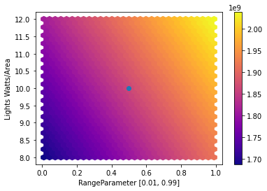
Interactive surrogate

Finally we make an interactive plot using ipywidgets, which executes the model every time a slider is moved.

# get the min and max of the two variables
(min1, max1), (min2, max2) = (
    (float(p.value_descriptor.min), p.value_descriptor.max) for p in problem.inputs
)
# get the data to plot in the background
df = run_model(model, 100)

# define a wrapper to be queried by interact
def model_wrapper(v1, v2):
    df.plot.hexbin(
        x=x, y=y, C=0, cmap="plasma", gridsize=30, sharex=False
    )  # background plot
    x_lims = plt.xlim()
    y_lims = plt.ylim()
    plt.scatter(x=v1, y=v2)  # plot the marker
    plt.xlim((x_lims))
    plt.ylim((y_lims))

    value = (
        model.predict([[v1, v2]])[0] / 3.6e6
    )  # find the current value and convert to kWh
    output = (
        "Electricity use = " + str(value.round()) + " kWh"
    )  # return the string to display
    return output


# make the interactive plot with two sliders
continuous_update = False
interact(
    model_wrapper,
    v1=FloatSlider(
        min=min1,
        max=max1,
        value=(min1 + max1) / 2,
        description="SHGC",
        step=0.01,
        continuous_update=continuous_update,
    ),
    v2=FloatSlider(
        min=min2,
        max=max2,
        value=(min2 + max2) / 2,
        description="LPD [W/m2]",
        continuous_update=continuous_update,
    ),
)

/usr/local/lib/python3.7/dist-packages/pandas/plotting/_matplotlib/tools.py:307: MatplotlibDeprecationWarning:
The rowNum attribute was deprecated in Matplotlib 3.2 and will be removed two minor releases later. Use ax.get_subplotspec().rowspan.start instead.
  layout[ax.rowNum, ax.colNum] = ax.get_visible()
/usr/local/lib/python3.7/dist-packages/pandas/plotting/_matplotlib/tools.py:307: MatplotlibDeprecationWarning:
The colNum attribute was deprecated in Matplotlib 3.2 and will be removed two minor releases later. Use ax.get_subplotspec().colspan.start instead.
  layout[ax.rowNum, ax.colNum] = ax.get_visible()
/usr/local/lib/python3.7/dist-packages/pandas/plotting/_matplotlib/tools.py:313: MatplotlibDeprecationWarning:
The rowNum attribute was deprecated in Matplotlib 3.2 and will be removed two minor releases later. Use ax.get_subplotspec().rowspan.start instead.
  if not layout[ax.rowNum + 1, ax.colNum]:
/usr/local/lib/python3.7/dist-packages/pandas/plotting/_matplotlib/tools.py:313: MatplotlibDeprecationWarning:
The colNum attribute was deprecated in Matplotlib 3.2 and will be removed two minor releases later. Use ax.get_subplotspec().colspan.start instead.
  if not layout[ax.rowNum + 1, ax.colNum]:

'Electricity use = 517.0 kWh'

<function __main__.model_wrapper(v1, v2)>