Building Optimization

This notebook performs building design optimization using EnergyPlus and BESOS helper functions. We load a model from in.idf, define parameters to vary, set objectives, test the model, then run a multi-objective genetic algorithm and plot the optimized designs.

Import libraries

import pandas as pd
from besos import eppy_funcs as ef, sampling
from besos.evaluator import EvaluatorEP
from besos.optimizer import NSGAII, df_solution_to_solutions
from besos.parameters import RangeDescriptor, expand_plist, wwr
from besos.problem import EPProblem
from matplotlib import pyplot as plt
from platypus import Archive, Hypervolume, Solution

Load the base EnergyPlus .idf file

building = ef.get_building("in.idf")

Define design parameters and ranges

Define a parameter list using a helper function, in this case building orientation and window-to-wall ratio.

parameters = []
parameters = expand_plist(
    {"Building 1": {"North Axis": (0, 359)}}  # Name from IDF Building object
)

parameters.append(
    wwr(RangeDescriptor(0.1, 0.9))
)  # Add window-to-wall ratio as a parameter between 0.1 and 0.9 using a custom function

Objectives

Using Heating and Cooling energy outputs as simulation objectives, make a problem instance from these parameters and objectives.

objectives = ["DistrictCooling:Facility", "DistrictHeating:Facility"]
besos_problem = EPProblem(parameters, objectives)

Set up EnergyPlus evaluator object to run simulations for this building and problem

evaluator = EvaluatorEP(
    besos_problem, building, out_dir="outputdir", err_dir="outputdir"
)  # outputdir must exist; E+ files will be written there
runs = pd.DataFrame.from_dict(
    {"0": [180, 0.5]}, orient="index"
)  # Make a dataframe of runs with one entry for South and 50% glazing
outputs = evaluator.df_apply(runs)  # Run this as a test
outputs

HBox(children=(FloatProgress(value=0.0, description='Executing', max=1.0, style=ProgressStyle(description_widt…

	DistrictCooling:Facility	DistrictHeating:Facility
0	3.233564e+09	4.931726e+09

Run the Genetic Algorithm

Run the optimizer using this evaluator for a population size of 20 for 10 generations.

results = NSGAII(evaluator, evaluations=10, population_size=20)
results

	North Axis	RangeDescriptor [0.1, 0.9]	DistrictCooling:Facility	DistrictHeating:Facility	violation	pareto-optimal
0	37.466568	0.779693	4.460085e+09	4.860635e+09	0	False
1	243.990689	0.467029	4.029894e+09	4.453658e+09	0	False
2	224.662175	0.685257	3.714934e+09	5.805083e+09	0	False
3	233.059795	0.400315	3.865349e+09	4.204440e+09	0	True
4	215.886962	0.681890	3.564599e+09	5.842255e+09	0	False
5	279.921039	0.867322	4.575077e+09	5.872849e+09	0	False
6	313.596088	0.405313	4.486791e+09	3.253404e+09	0	False
7	348.248353	0.101710	4.358378e+09	1.701099e+09	0	True
8	132.035405	0.467023	3.716682e+09	4.654626e+09	0	True
9	269.248373	0.530728	4.365569e+09	4.459456e+09	0	False
10	350.161374	0.347721	4.284927e+09	2.703139e+09	0	False
11	234.224202	0.602762	3.879037e+09	5.255264e+09	0	False
12	89.948274	0.145898	4.234634e+09	2.592709e+09	0	True
13	180.197818	0.541119	3.221832e+09	5.150586e+09	0	True
14	294.747583	0.414158	4.490630e+09	3.517963e+09	0	False
15	318.608866	0.467363	4.479668e+09	3.453551e+09	0	False
16	350.864950	0.762852	4.326616e+09	4.475655e+09	0	False
17	186.068791	0.562011	3.231265e+09	5.262056e+09	0	False
18	13.197950	0.758258	4.309214e+09	4.462021e+09	0	False
19	46.755428	0.818880	4.519118e+09	5.201453e+09	0	False

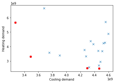
Visualize the results

optres = results.loc[
    results["pareto-optimal"] == True, :
]  # Get only the optimal results
plt.plot(
    results["DistrictCooling:Facility"], results["DistrictHeating:Facility"], "x"
)  # Plot all results in the background as blue crosses
plt.plot(
    optres["DistrictCooling:Facility"], optres["DistrictHeating:Facility"], "ro"
)  # Plot optimal results in red
plt.xlabel("Cooling demand")
plt.ylabel("Heating demand")

Text(0, 0.5, 'Heating demand')

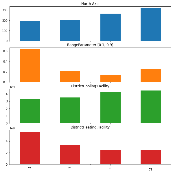
optres = optres.sort_values("DistrictCooling:Facility")  # Sort by the first objective
optresplot = optres.drop(columns="violation")  # Remove the constraint violation column
ax = optresplot.plot.bar(
    subplots=True, legend=None, figsize=(10, 10)
)  # Plot the variable values of each of the optimal solutions

/usr/local/lib/python3.7/dist-packages/pandas/plotting/_matplotlib/tools.py:307: MatplotlibDeprecationWarning:
The rowNum attribute was deprecated in Matplotlib 3.2 and will be removed two minor releases later. Use ax.get_subplotspec().rowspan.start instead.
  layout[ax.rowNum, ax.colNum] = ax.get_visible()
/usr/local/lib/python3.7/dist-packages/pandas/plotting/_matplotlib/tools.py:307: MatplotlibDeprecationWarning:
The colNum attribute was deprecated in Matplotlib 3.2 and will be removed two minor releases later. Use ax.get_subplotspec().colspan.start instead.
  layout[ax.rowNum, ax.colNum] = ax.get_visible()
/usr/local/lib/python3.7/dist-packages/pandas/plotting/_matplotlib/tools.py:313: MatplotlibDeprecationWarning:
The rowNum attribute was deprecated in Matplotlib 3.2 and will be removed two minor releases later. Use ax.get_subplotspec().rowspan.start instead.
  if not layout[ax.rowNum + 1, ax.colNum]:
/usr/local/lib/python3.7/dist-packages/pandas/plotting/_matplotlib/tools.py:313: MatplotlibDeprecationWarning:
The colNum attribute was deprecated in Matplotlib 3.2 and will be removed two minor releases later. Use ax.get_subplotspec().colspan.start instead.
  if not layout[ax.rowNum + 1, ax.colNum]:

Hypervolume

Now that initial results have been produced and verified against expectations, enlarge evaluations and population size to produce increased optimization of results.

results_2 = NSGAII(evaluator, evaluations=20, population_size=50)

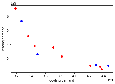
Compare first run and second run

optres_2 = results_2.loc[results_2["pareto-optimal"] == True, :]
plt.plot(
    optres["DistrictCooling:Facility"], optres["DistrictHeating:Facility"], "bo"
)  # Plot first optimal results in blue
plt.plot(
    optres_2["DistrictCooling:Facility"], optres_2["DistrictHeating:Facility"], "ro"
)  # Plot second optimal results in red
plt.xlabel("Cooling demand")
plt.ylabel("Heating demand")

Text(0, 0.5, 'Heating demand')

Calculate the hypervolume

reference_set = Archive()
platypus_problem = evaluator.to_platypus()
for _ in range(20):
    solution = Solution(platypus_problem)
    solution.variables = sampling.dist_sampler(
        sampling.lhs, besos_problem, 1
    ).values.tolist()[0]
    solution.evaluate()
    reference_set.add(solution)

hyp = Hypervolume(reference_set)
print(
    "Hypervolume for result 1:",
    hyp.calculate(df_solution_to_solutions(results, platypus_problem, besos_problem)),
)
print(
    "Hypervolume for result 2:",
    hyp.calculate(df_solution_to_solutions(results_2, platypus_problem, besos_problem)),
)

Hypervolume for result 1: 0.5044186053393032
Hypervolume for result 2: 0.6217620026588312